


Constructing global physical input-output tables for iron and steel
Hanspeter Wieland & Stefan Giljum
FINEPRINT Brief No. 7, August 2019
The supply chains of iron and steel are highly globalised and constantly expanding. Current models have limitations in depicting the complex physical reality in high product and geographical detail. In this Brief, we describe the FINEPRINT approach to model global iron and steel flows based on physical input-output tables. The current model differentiates 21 iron and steel commodities for 34 countries and a rest of the world region, interlinked through international trade. The Brief showcases first results to highlight the analytical possibilities and gives an outlook to future developments.
Iron ores are strategically important resources for industrialised and industrialising societies and their extraction is regarded as one of the most environmentally disruptive activities undertaken by business. The iron and steel sector was the largest industrial emitter of CO2 in 2015, accounting for approximately 30% of global CO2 emissions from industries. Trade plays a crucial role in securing the supply of countries without domestic extraction. In 2015, only five countries (BRIC + Australia) accounted for 85% of global iron ore extraction. The intensifying spatial disconnect between extractors, processors and users, unprecedented growth rates of global extraction (ca. 9% p.a.) and the threefold increase of trade volumes since 1995, signify a highly dynamic global iron-steel (I-S) supply chain network. This network is going through profound structural change, involving higher levels of interdependence and connectivity between world regions and industries.
Multi-regional input-output (MRIO) databases extended with environmental data are frequently applied for the analysis of metal supply chains [1]. These models combine two elements: an input-output (IO) table representing monetary inter-industry flows of intermediate inputs and final demand, and an extension table in physical units depicting environmental flows that are associated with economic activities. Conceptually, extension tables describe flows required for economic activities that are not directly captured by the monetary IO table. In environmental terms, this corresponds to boundary flows entering (e.g. inputs from nature) or leaving (e.g. greenhouse gas emissions) the economy. MRIO tables are mostly available only in monetary units, thereby assuming proportionality between monetary and physical flows. This does not always represent the reality of physical flows due to price inhomogeneities. Furthermore, the first processing steps of metal ores are highly aggregated in monetary tables, thereby impeding more detailed assessments of the first transformation processes in metal supply chains. Physical IO tables (PIOT) on the other hand are usually only available for single countries. Quantifying metal cycles is a basic aim in material flow analysis (MFA), but the global models usually lack geographical detail and markets are not always trade-linked [2,3]. Moreover, physical data on metal flows from the intermediate stage to end-use are scarce.
Against this background, our modelling approach brings together the advantages of different modelling fields, combining the strengths of physical assessments of high product detail with the opportunities to perform global analyses of high geographical detail. Before going into more details of the modelling approach, the following section describes the central characteristics of the multi-regional PIOT.
The system structure of the PIOT
Figure 1 shows the layout of the iron and steel PIOT, which follows the general guidelines and system structure as set forth by the UN System of Environmental and Economic Accounting (SEEA). In its current form, the tables include data for 34 countries plus a rest of the world region. International trade flows are depicted in the off-diagonal blocks, shown in light blue and light red in Figure 1. The PIOT differentiates between 21 commodities of iron and steel and three boundary flows, i.e. inputs from nature and end-of-life scrap as well as wastes. Out of the 21 commodities, 11 refer to intermediate inputs (e.g., iron ores, semi-finished billets or finished steel in the form of flat rolled products) and 10 to commodities for final use (e.g., the amount of steel that is contained in machinery or transport equipment). Columns of the table reflect inputs into production processes and rows depict outputs and the distribution thereof on (global) markets, including wastes that are ultimately discarded back to the environment (e.g., unrecoverable iron oxides in slag). The construction of the PIOT follows the mass balance principle. Summing over a column (inputs) therefore must match the sum over the corresponding row (output), i.e. total output.
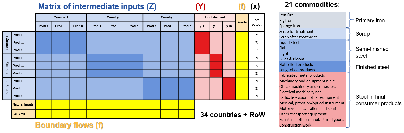
Figure 1: Structure of the physical IO tables for iron and steel
The modelling framework
The general idea of the iron and steel model developed in FINEPRINT is to integrate two separately constructed modules, each describing the flows at different stages of the iron-steel supply chain.
The first module reflects flows from extraction via processing and fabrication to manufacturing (the blue intermediate matrix in Figure 1). Informed by existing MFA studies [2], we designed a global trade-linked material flow model of iron and steel, based on supply and use tables, to capture the first (intermediate) steps of the supply chain. Production amounts for different countries and processes (e.g., blast oxygen or electric arc furnaces) are reported in the statistical yearbooks of the Worldsteel Association. Information on average yields and efficiencies in steelmaking were collected form technical reports, for example, from the Worldsteel Association, and the scientific literature. Trade data was sourced from the BACI i.e. Comtrade database. The products with the highest degree of fabrication that are captured by this module are intermediate products (e.g. finished steel like flat or long rolled products), which will be used by manufacturing processes further downstream.
The second module reflects flows from manufacturing to final demand and is constructed applying a hybrid IO modelling technique, i.e. the waste input-output (WIO) approach to material flows [4]. The WIO approach allows deriving a physical flow matrix from existing MRIOs. A filter matrix (with zeros and ones) is used to remove monetary flows from the MRIO table that allegedly do not correspond to apparent physical quantities. Using the filtered IO table, outputs of module 1 (finished steel products) are allocated to final demand. We apply the MRIO-database EXIOBASE for setting up the WIO module due to the high level of product disaggregation. The WIO approach delivers a multi-regional physical flow table, covering higher manufacturing and end use. Combining tables from module 1 and module 2 results in a global PIOT, containing all physical flows from mining of iron ores to final products, including waste streams and secondary metal (scrap).
PIOT-based material flow indicators
Using China and the year 2014 as an example, Figure 2 provides an overview of the different material flow indicators that can be calculated from the PIOT. Due to the mass balance principle, all indicators are consistent with each other. On the one hand, we can derive material flow indicators that focus on the production-based perspective, describing apparent/direct flows within the territory of a country (left side of Figure 2). Summation of all boundary inputs gives the domestic supply of iron ore (inputs from nature) and steel (End-of-Life scrap). Physical imports to and exports from a specific country are calculated by summing over the respective columns and rows. Domestic Material Consumption (DMC) is the sum of a countries’ final demand and all the wastes produced on its territory.
When using the Leontief inverse, we can also take a consumption-based perspective that quantifies the upstream or embodied material use that is indirectly required to satisfy final demand in a country. This allows quantifying Raw Material Equivalents (RME) of trade flows or different types of Raw Material Consumption (RMC) indicators, i.e. material footprints. RMC-Supply measures all boundary inputs (inputs form nature and EoL scrap) required to produce goods for final demand and RMC-Use the final demand plus all boundary outputs (wastes). Again, due to the mass balance principle, both indicators must add up to the same total.
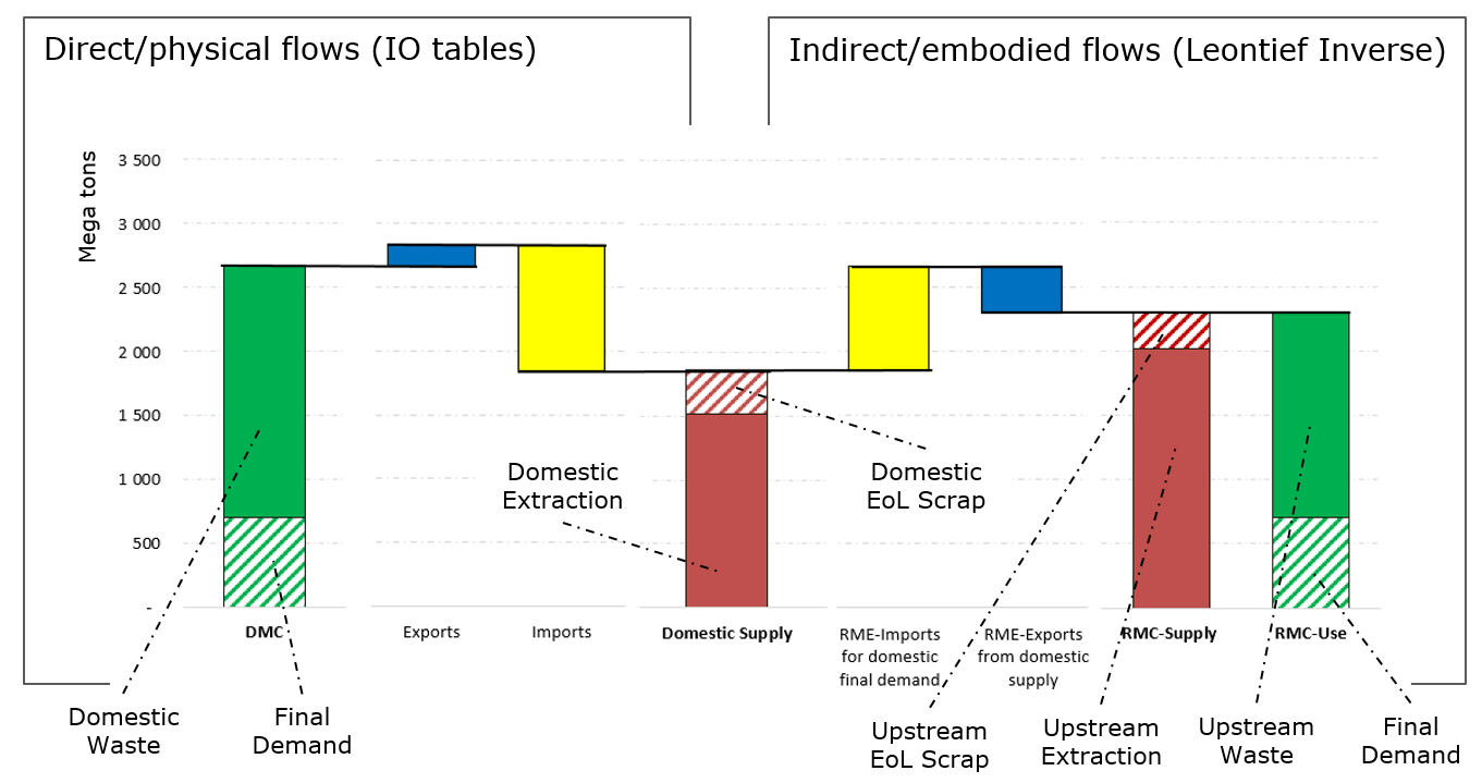
Figure 2: A set of consistent material flow indicators for China in 2014, derived from the global iron and steel PIOT
The results for China 2014 reveal that about 40% of the extracted iron ore that serves final demand originates from abroad (compare RME-Imports and RMC-Supply in Figure 2). Moreover, almost 20% of Chinas domestic waste production (which is mostly waste rock) is not associated with final demand within the country, but with production of exports (compare domestic waste flows and upstream waste). In terms of direct flow indicators, China is a net-importer (DMC > DE), but a net-exporter regarding indirect (embodied) waste flows (DMC > RMC-Use). This is a result of China’s position in the global economic system. China imports large amounts of iron ores and processes them into products, which are partly re-exported, while generating waste flows within China.
Network analyses of global supply chains
We can also use the PIOT database to perform a network analysis of the global physical trade networks. The 21 commodities are aggregated into five distinct layers, i.e. primary iron, scrap, semi-finished steel, finished steel and steel in final consumer products. Each layer reflects different stages of the iron-steel supply chains.
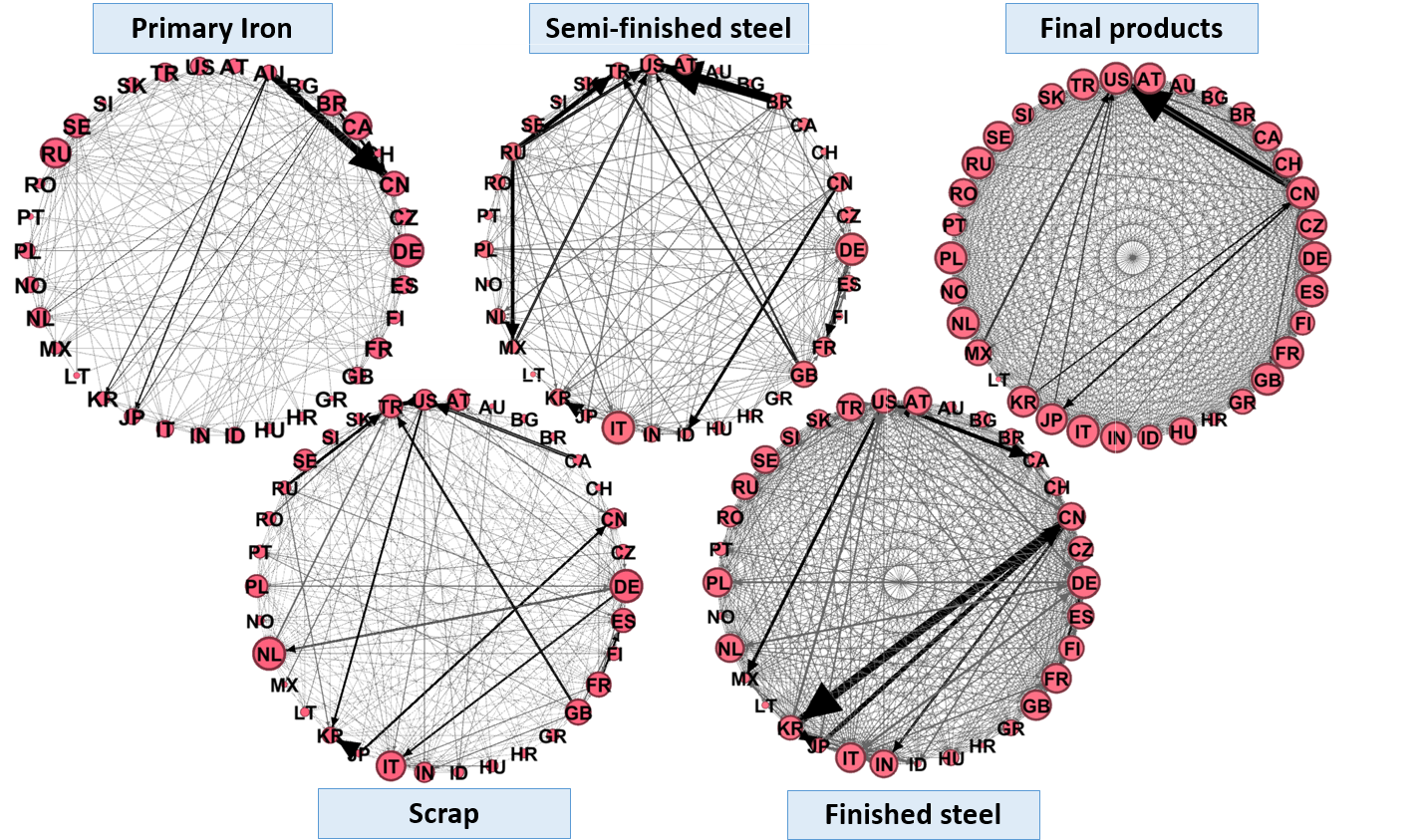
Figure 3: Network graphs showing international trade flows of the 34 countries of the 2014 PIOT for different layers (product groups) of iron and steel supply chains
Using these five layers of iron and steel, we can measure the density of the physical trade networks. The results show that the density of trade networks tends to increase with the degree of processing. Primary iron, the initial layer/stage of the supply chain, is the least dense network: only 19% of the theoretically possible trade relations between all partners are actually realised. Exports from Australia (AU) to China (CN) are the single largest trade flow. The scrap trade network has a density of 31% and countries such as Turkey (TR), Korea (KR) and Germany (DE) have particularly large imports. The semi-finished steel network has a density of 23%, where the most important actors are Brazil (BR), United States (US) and Russia (RU). Trade networks of finished steel and final products are the densest layers with 72% and 92% respectively. China again is a key actor here, exporting large amounts of finished steel to Korea and steel in final consumer products to the United States. We can also calculate the number of bilateral trade relations each country maintains, which is the number of import links plus the number of export links i.e. in-degree and out-degree. The size of the red bubbles of the countries reflects this measure. In Figure 3, it can be seen that Germany (DE) holds a large number of bilateral trade relations across all layers of the supply chain, reflecting Germany’s strong embeddedness in global supply chains and large exports in sectors such as machinery or vehicles.
Outlook
We will follow up several directions of further developments of the iron and steel PIOT. As one important next step, we aim at increasing the number of countries by means of a uniform estimation procedure that allows quantifying production values for those countries where available data sources are incomplete or insufficient. Another step is to disaggregate different product groups by adding more detailed information from the statistical yearbooks. This involves for example breaking down finished steel (flat and long rolled products) into different sub-groups, such as concrete reinforcing bars or wire rod. We will also disaggregate ‘liquid steel’ into two different types, in order to allow for a better representation of the primary (from iron ores) and the secondary (from scrap) route in steelmaking. At the moment, boundary flows of End-of-Life scrap and wastes are treated as balancing items in the compilation of the PIOT. In this regard the next step is to make use of dynamic material flow model results on countries’ EoL steel scrap flows, in conjunction with a constrained optimisation tool [5] to obtain a better estimate of these flows. In the medium term, we plan to compile different extension tables for the PIOT (e.g., water, land, energy or greenhouse gases) that can be used to calculate footprint-type indicators and perform nexus analyses for different resource categories.
Citation
Wieland, H., Giljum, S., 2019. Constructing global physical input-output tables for iron and steel. FINEPRINT Brief No. 7. Vienna University of Economics and Business (WU). Austria
References
[1] Moran D, McBain D, Kanemoto K, Lenzen M, Geschke A. Global supply chains of coltan. Journal of Industrial Ecology 2015;19:357–65. doi:10.1111/jiec.12206.
[2] Cullen JM, Allwood JM, Bambach MD. Mapping the global flow of steel: From steelmaking to end-use goods. Environmental Science & Technology 2012;46:13048–55. doi:10.1021/es302433p.
[3] Pauliuk S, Wang T, Müller DB. Steel all over the world: Estimating in-use stocks of iron for 200 countries. Resources, Conservation and Recycling 2013;71:22–30. doi:10.1016/j.resconrec.2012.11.008.
[4] Nakamura S, Nakajima K, Kondo Y, Nagasaka T. The waste input-output approach to materials flow analysis. Journal of Industrial Ecology 2007;11:50–63. doi:10.1162/jiec.2007.1290.
[5] Geschke A, Wood R, Kanemoto K, Lenzen M, Moran D. Investigating alternative approaches to harmonise multi-regional input-output data. Economic Systems Research 2014;26:354–85.